Deep Learning and Neural Network
Deep learning (DL) is simply one of many available frameworks for deciphering machine learning problems. Deep models are termed “deep” as there are multiple computation layers. In the past, the important part of ML application consisted of putting in manually engineered methods of transforming a given data into a form suitable to shallow models.
The key advantage of deep learning is the replacement of not only the shallow models at traditional learning pipelines, but also the labour-intensive feature engineering. Deep learning also replaces a major chunk of domain-specific pre-processing. Deep learning has eliminated the boundaries that previously demarcated computer vision, medical informatics, natural language processing, and speech recognition. DL offers a unified toolset for managing diverse problems.
Machine Learning (ML) uses data to ascertain transformations among inputs and outputs, like harvesting text from audio in speech recognition. To do so, it is frequently necessary to depict data in such a manner that the algorithms can change such depictions into output. Deep learning (DL) is deep in the sense that its models assimilate multiple layers of transformations, and where every individual layer provides representation at that level. To give an example, layers close to the input may depict low-level features of that data, while layers nearer to classification output may depict additional discriminatory abstract concepts. Since the goal of representation learning is to find the representation itself, DL may also be termed as multi-level representation learning.
Building Intelligent Machines (The Neural Network)
Deep learning refers to learning networks with many layers of neurons. Neuron is the human brain's foundational unit. A brain fragment, akin to a rice grain, packs approximately 10,000 neurons. Each neuron forms about 6,000 interconnections with other neurons.
Industrial maintenance is classified into different types:
Neuron
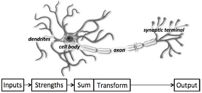
An individual neuron, at its core, is optimized to accept information from other neurons, and uniquely process such details. The result is then dispatched to other cells. The receiving neuron acquires its inputs along the dendrites (antenna-like structures). Each dendrite is dynamically weakened or strengthened based on the frequency of its use.

Figure 1: A functional description of a biological neuron’s structure
The individual strength connection determines the contributory input to that neuron's output. The inputs, after they are weighted by the robustness of their corresponding connections, are totted up inside the cell body. The sum is then converted to a new signal which consequently transmits down the cell's axon and ultimately dispatched to other neurons.
Artificial Neuron
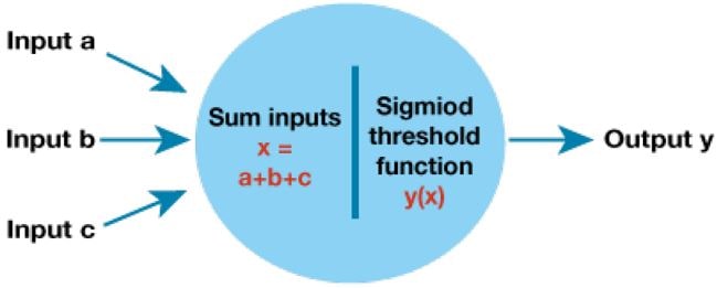
Such functional understanding of our brain neurons can be translated into a computer depictive artificial model. The artificial neuron, similar to a biological neuron receives a few inputs, x1, x2, . . . , xn. The individual input is then multiplied by a particular weight, w1,w2, . . . ,wn. Such weighted inputs are then summed together to generate the neuron logit,  . In many instances, the logit also comprises a bias - a constant (not in figure). This logit is then sent through a function f to generate the output y = f z. Such an output is possible to be conveyed to other neurons.

Figure 2: Schematic for a neuron in an artificial neural net
This mathematical treatise of the artificial neuron can be concluded through re-expressing its functionality in the vector form. The inputs can be reformulated as vector x = [x1, x2, . . . , xn] neuron weights as w = [w1,w2, . . . ,wn]. We can now re-express the neuron output as y = f (x ・w + b), where b refers to the bias term. To put it differently, we can calculate the output by executing the dot product of weight and input vectors, added into the bias term to generate the logit, and subsequently applying the all-important transformation function.
Following a Signal Through a Neural Network
The following illustration explains a smaller, two-layer neural network, with each layer having two neurons:

Let’s assume the two inputs are 1.0 and 0.5. These inputs are entered into this smaller neural network.
A few random weights are assumed:
W1,1=0.9, W1,2=0.2, W2,1= 0.3, W2,2= 0.8
It is now prudent to calculate the output of both inputs. The output x is given as
X = (output from first node * link weight) + (output from second node* link weight)
X1= (1.0 * 0.9) + (0.5 * 0.3) =1.05
X2= (1.0 * 0.2) + (0.5 * 0.8) =0.6
Applying the sigmoid function

we get
Y(X1) =1/ (1+0.34993) =1/ (1.34993) =0.7408
Y(X2) = 1/ (1 + 0.5488) = 1/ (1.5488) = 0.6457
These simple calculations will be too complicated for a network comprised of 5 layers and 100 nodes in every layer. Matrices can solve this puzzle. The above calculation can be written in matrix form as:

Let us see a simple neural network program in python:
from numpy import exp, array, random, dot
class NeuralNetwork():
def __init__(self):
random.seed(1)
random.seed(1)self.synaptic_weights = 2 * random.random((3, 1)) - 1
def __sigmoid(self, x):
return 1 / (1 + exp(-x))
def __sigmoid_derivative(self, x):
return x * (1 - x)
def train(self, training_set_inputs, training_set_outputs, number_of_training_iterations):
for iteration in xrange(number_of_training_iterations):
output = self.think(training_set_inputs)
error = training_set_outputs - output
adjustment = dot(training_set_inputs.T, error * self.__sigmoid_derivative(output))
self.synaptic_weights += adjustment
def think(self, inputs):
return self.__sigmoid(dot(inputs, self.synaptic_weights))
if __name__ == "__main__":
neural_network = NeuralNetwork()
print "Random weights: "
print neural_network.synaptic_weights
training_set_inputs = array([[0, 0, 1], [1, 1, 1], [1, 0, 1], [0, 1, 1]])
training_set_outputs = array([[0, 1, 1, 0]]).T
neural_network.train(training_set_inputs, training_set_outputs, 10000)
print "New synaptic weights: "
print neural_network.synaptic_weights
print neural_network.think(array([1, 0, 0]))
The above neural network program can be run on many single board computers. The Raspberry Pi and Beagle Bone AI comes with pre compiled linux operating systems such as Raspbian and Debian which is very well suited for the beginners. The other single board computer such as AM437X ARM Cortex-A9, MaaXBoard AES-MC-SBC-IMX8M-G and SBC-S32V234 does not come with a pre-built operating system and the user has to compile the Linux operating from scratch. Although these are good for learning and for hobbyist, they are not targeted for the beginners.
If any hobbyist wants the power of FPGA along with ARM, they can opt for the Ultra96-V2 board.
Stay informed
Keep up to date on the latest information and exclusive offers!
Subscribe now
Thanks for subscribing
Well done! You are now part of an elite group who receive the latest info on products, technologies and applications straight to your inbox.
Related Articles
- Advanced ML for MEMS Sensors: Enhancing the Accuracy, Performance, and Power consumption
- How to design a MEMS Vibration Sensor for predictive maintenance
- Precision in Sight: How AI-powered visual inspection improves industrial quality control
- How to Capture High-Quality, Undistorted Images for Industrial Machine Vision
- Robotics and AI Integration: Transforming Industrial Automation
- The modern challenges of facial recognition
- Intelligent cameras for smart security and elevated surveillance
- Evolution of voice, speech, and sound recognition
- AI and IoT: The future of intelligent transportation systems
- Machine Vision Sensors: How Machines View the World
- Demystifying AI and ML with embedded devices
- How to implement convolutional neural network on STM32 and Arduino
- How to do image classification using ADI MAX78000
- The Benefits of Using Sensors and AI in HVAC Systems
- Deep learning and neural networks
- Latest Trends in Artificial Intelligence
- Hello world for Machine Learning
- How to implement AR in process control application


